Attentions

This notebook explains how to get various attention images with Saliency, SmoothGrad, GradCAM, GradCAM++ and ScoreCAM/Faster-ScoreCAM.

Preparation

Load libraries

[1]:

%reload_ext autoreload
%autoreload 2
import warnings

warnings.filterwarnings('ignore')

import numpy as np
import tensorflow as tf
from matplotlib import pyplot as plt

%matplotlib inline
from packaging.version import parse as version

from tf_keras_vis.utils import num_of_gpus

if version(tf.version.VERSION) < version('2.16.0'):
    import tensorflow.keras as keras
else:
    import keras

_, gpus = num_of_gpus()
print('Tensorflow recognized {} GPUs'.format(gpus))

2025-03-12 12:09:03.983745: E external/local_xla/xla/stream_executor/cuda/cuda_fft.cc:477] Unable to register cuFFT factory: Attempting to register factory for plugin cuFFT when one has already been registered
WARNING: All log messages before absl::InitializeLog() is called are written to STDERR
E0000 00:00:1741748944.092840     819 cuda_dnn.cc:8310] Unable to register cuDNN factory: Attempting to register factory for plugin cuDNN when one has already been registered
E0000 00:00:1741748944.124880     819 cuda_blas.cc:1418] Unable to register cuBLAS factory: Attempting to register factory for plugin cuBLAS when one has already been registered
2025-03-12 12:09:04.364544: I tensorflow/core/platform/cpu_feature_guard.cc:210] This TensorFlow binary is optimized to use available CPU instructions in performance-critical operations.
To enable the following instructions: AVX2 AVX512F AVX512_VNNI FMA, in other operations, rebuild TensorFlow with the appropriate compiler flags.

Tensorflow recognized 0 GPUs

2025-03-12 12:09:10.701446: E external/local_xla/xla/stream_executor/cuda/cuda_driver.cc:152] failed call to cuInit: INTERNAL: CUDA error: Failed call to cuInit: CUDA_ERROR_NO_DEVICE: no CUDA-capable device is detected

Load keras.Model

In this notebook, we use VGG16 model, but if you want to use other keras.Model, you can do so by modifying the section below.

[2]:

model = keras.applications.vgg16.VGG16(weights='imagenet', include_top=True)
model.summary()

Model: "vgg16"

┏━━━━━━━━━━━━━━━━━━━━━━━━━━━━━━━━━┳━━━━━━━━━━━━━━━━━━━━━━━━┳━━━━━━━━━━━━━━━┓
┃ Layer (type)                    ┃ Output Shape           ┃       Param # ┃
┡━━━━━━━━━━━━━━━━━━━━━━━━━━━━━━━━━╇━━━━━━━━━━━━━━━━━━━━━━━━╇━━━━━━━━━━━━━━━┩
│ input_layer (InputLayer)        │ (None, 224, 224, 3)    │             0 │
├─────────────────────────────────┼────────────────────────┼───────────────┤
│ block1_conv1 (Conv2D)           │ (None, 224, 224, 64)   │         1,792 │
├─────────────────────────────────┼────────────────────────┼───────────────┤
│ block1_conv2 (Conv2D)           │ (None, 224, 224, 64)   │        36,928 │
├─────────────────────────────────┼────────────────────────┼───────────────┤
│ block1_pool (MaxPooling2D)      │ (None, 112, 112, 64)   │             0 │
├─────────────────────────────────┼────────────────────────┼───────────────┤
│ block2_conv1 (Conv2D)           │ (None, 112, 112, 128)  │        73,856 │
├─────────────────────────────────┼────────────────────────┼───────────────┤
│ block2_conv2 (Conv2D)           │ (None, 112, 112, 128)  │       147,584 │
├─────────────────────────────────┼────────────────────────┼───────────────┤
│ block2_pool (MaxPooling2D)      │ (None, 56, 56, 128)    │             0 │
├─────────────────────────────────┼────────────────────────┼───────────────┤
│ block3_conv1 (Conv2D)           │ (None, 56, 56, 256)    │       295,168 │
├─────────────────────────────────┼────────────────────────┼───────────────┤
│ block3_conv2 (Conv2D)           │ (None, 56, 56, 256)    │       590,080 │
├─────────────────────────────────┼────────────────────────┼───────────────┤
│ block3_conv3 (Conv2D)           │ (None, 56, 56, 256)    │       590,080 │
├─────────────────────────────────┼────────────────────────┼───────────────┤
│ block3_pool (MaxPooling2D)      │ (None, 28, 28, 256)    │             0 │
├─────────────────────────────────┼────────────────────────┼───────────────┤
│ block4_conv1 (Conv2D)           │ (None, 28, 28, 512)    │     1,180,160 │
├─────────────────────────────────┼────────────────────────┼───────────────┤
│ block4_conv2 (Conv2D)           │ (None, 28, 28, 512)    │     2,359,808 │
├─────────────────────────────────┼────────────────────────┼───────────────┤
│ block4_conv3 (Conv2D)           │ (None, 28, 28, 512)    │     2,359,808 │
├─────────────────────────────────┼────────────────────────┼───────────────┤
│ block4_pool (MaxPooling2D)      │ (None, 14, 14, 512)    │             0 │
├─────────────────────────────────┼────────────────────────┼───────────────┤
│ block5_conv1 (Conv2D)           │ (None, 14, 14, 512)    │     2,359,808 │
├─────────────────────────────────┼────────────────────────┼───────────────┤
│ block5_conv2 (Conv2D)           │ (None, 14, 14, 512)    │     2,359,808 │
├─────────────────────────────────┼────────────────────────┼───────────────┤
│ block5_conv3 (Conv2D)           │ (None, 14, 14, 512)    │     2,359,808 │
├─────────────────────────────────┼────────────────────────┼───────────────┤
│ block5_pool (MaxPooling2D)      │ (None, 7, 7, 512)      │             0 │
├─────────────────────────────────┼────────────────────────┼───────────────┤
│ flatten (Flatten)               │ (None, 25088)          │             0 │
├─────────────────────────────────┼────────────────────────┼───────────────┤
│ fc1 (Dense)                     │ (None, 4096)           │   102,764,544 │
├─────────────────────────────────┼────────────────────────┼───────────────┤
│ fc2 (Dense)                     │ (None, 4096)           │    16,781,312 │
├─────────────────────────────────┼────────────────────────┼───────────────┤
│ predictions (Dense)             │ (None, 1000)           │     4,097,000 │
└─────────────────────────────────┴────────────────────────┴───────────────┘

 Total params: 138,357,544 (527.79 MB)

 Trainable params: 138,357,544 (527.79 MB)

 Non-trainable params: 0 (0.00 B)

Load and preprocess images

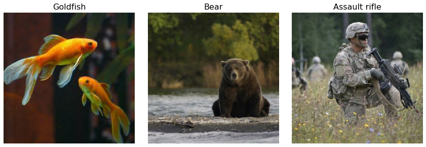
tf-keras-vis supports batch-wise visualization. Here, we load and preprocess three pictures of goldfish, bear and assault-rifle as input data.

[3]:

# Image titles
image_titles = ['Goldfish', 'Bear', 'Assault rifle']

# Load images and Convert them to a Numpy array
img1 = keras.preprocessing.image.load_img('images/goldfish.jpg', target_size=(224, 224))
img2 = keras.preprocessing.image.load_img('images/bear.jpg', target_size=(224, 224))
img3 = keras.preprocessing.image.load_img('images/soldiers.jpg', target_size=(224, 224))
images = np.asarray([np.array(img1), np.array(img2), np.array(img3)])

# Preparing input data for VGG16
X = keras.applications.vgg16.preprocess_input(images)

# Rendering
f, ax = plt.subplots(nrows=1, ncols=3, figsize=(12, 4))
for i, title in enumerate(image_titles):
    ax[i].set_title(title, fontsize=16)
    ax[i].imshow(images[i])
    ax[i].axis('off')
plt.tight_layout()
plt.show()

Implement functions required to use attentions

Model modifier

When the softmax activation function is applied to the last layer of model, it may obstruct generating the attention images, so you should replace the function to a linear activation function. Although we create and use ReplaceToLinear instance here, we can also use the model modifier function defined by ourselves.

[4]:

from tf_keras_vis.utils.model_modifiers import ReplaceToLinear

replace2linear = ReplaceToLinear()


# Instead of using the ReplaceToLinear instance above,
# you can also define the function from scratch as follows:
def model_modifier_function(cloned_model):
    cloned_model.layers[-1].activation = keras.activations.linear

Score function

And then, you MUST create Score instance or define score function that returns target scores. Here, they return the score values corresponding Goldfish, Bear, Assault Rifle.

[5]:

from tf_keras_vis.utils.scores import CategoricalScore

# 1 is the imagenet index corresponding to Goldfish, 294 to Bear and 413 to Assault Rifle.
score = CategoricalScore([1, 294, 413])


# Instead of using CategoricalScore object,
# you can also define the function from scratch as follows:
def score_function(output):
    # The `output` variable refers to the output of the model,
    # so, in this case, `output` shape is `(3, 1000)` i.e., (samples, classes).
    return (output[0][1], output[1][294], output[2][413])

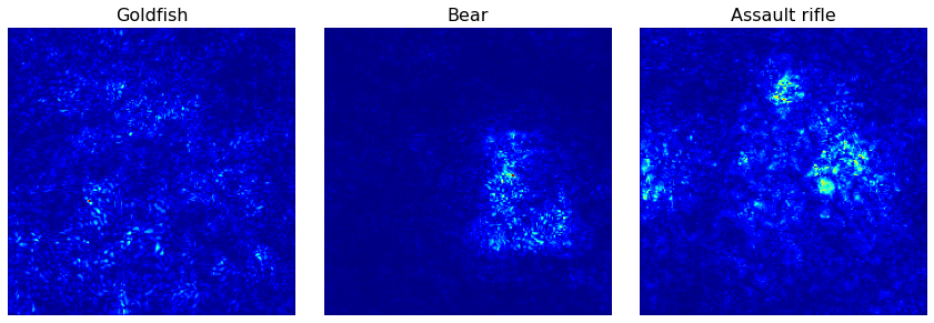
Vanilla Saliency

Saliency generates a saliency map that appears the regions of the input image that contributes the most to the output value.

[6]:

%%time
from tf_keras_vis.saliency import Saliency

# from tf_keras_vis.utils import normalize

# Create Saliency object.
saliency = Saliency(model, model_modifier=replace2linear, clone=True)

# Generate saliency map
saliency_map = saliency(score, X)

# Render
f, ax = plt.subplots(nrows=1, ncols=3, figsize=(12, 4))
for i, title in enumerate(image_titles):
    ax[i].set_title(title, fontsize=16)
    ax[i].imshow(saliency_map[i], cmap='jet')
    ax[i].axis('off')
plt.tight_layout()
plt.show()

CPU times: user 11.9 s, sys: 1.03 s, total: 12.9 s
Wall time: 2.97 s

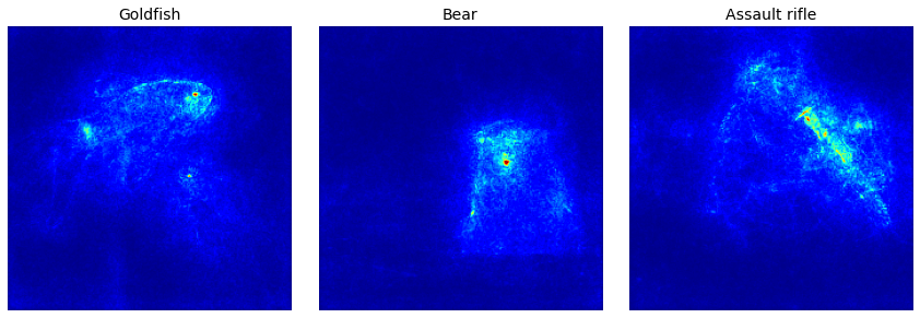
SmoothGrad

As you can see above, Vanilla Saliency map is too noisy, so let’s remove noise in the saliency map using SmoothGrad! SmoothGrad is a method that reduce the noise in saliency map by adding noise to input image.

Note: Because SmoothGrad calculates the gradient repeatedly, it might take much time around 2-3 minutes when using CPU.

[7]:

%%time

# Generate saliency map with smoothing that reduce noise by adding noise
saliency_map = saliency(
    score,
    X,
    smooth_samples=20,  # The number of calculating gradients iterations.
    smooth_noise=0.20)  # noise spread level.

# Render
f, ax = plt.subplots(nrows=1, ncols=3, figsize=(12, 4))
for i, title in enumerate(image_titles):
    ax[i].set_title(title, fontsize=14)
    ax[i].imshow(saliency_map[i], cmap='jet')
    ax[i].axis('off')
plt.tight_layout()
plt.savefig('images/smoothgrad.png')
plt.show()

CPU times: user 3min 30s, sys: 7.11 s, total: 3min 38s
Wall time: 35.7 s

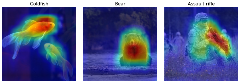
GradCAM

Saliency is one of useful way of visualizing attention that appears the regions of the input image that contributes the most to the output value. GradCAM is another way of visualizing attention over input. Instead of using gradients of model outputs, it uses of penultimate layer output (that is the convolutional layer just before Dense layers).

[8]:

%%time

from matplotlib import cm

from tf_keras_vis.gradcam import Gradcam

# Create Gradcam object
gradcam = Gradcam(model, model_modifier=replace2linear, clone=True)

# Generate heatmap with GradCAM
cam = gradcam(score, X, penultimate_layer=-1)

# Render
f, ax = plt.subplots(nrows=1, ncols=3, figsize=(12, 4))
for i, title in enumerate(image_titles):
    heatmap = np.uint8(cm.jet(cam[i])[..., :3] * 255)
    ax[i].set_title(title, fontsize=16)
    ax[i].imshow(images[i])
    ax[i].imshow(heatmap, cmap='jet', alpha=0.5)  # overlay
    ax[i].axis('off')
plt.tight_layout()
plt.show()

CPU times: user 12.5 s, sys: 2.06 s, total: 14.6 s
Wall time: 3.18 s

As you can see above, GradCAM is useful method for intuitively knowing where the attention is. However, when you take a look closely, you’ll see that the visualized attentions don’t completely cover the target (especially the head of Bear) in the picture.

Okay then, let’s move on to next method that is able to fix the problem above you looked.

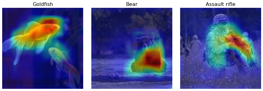
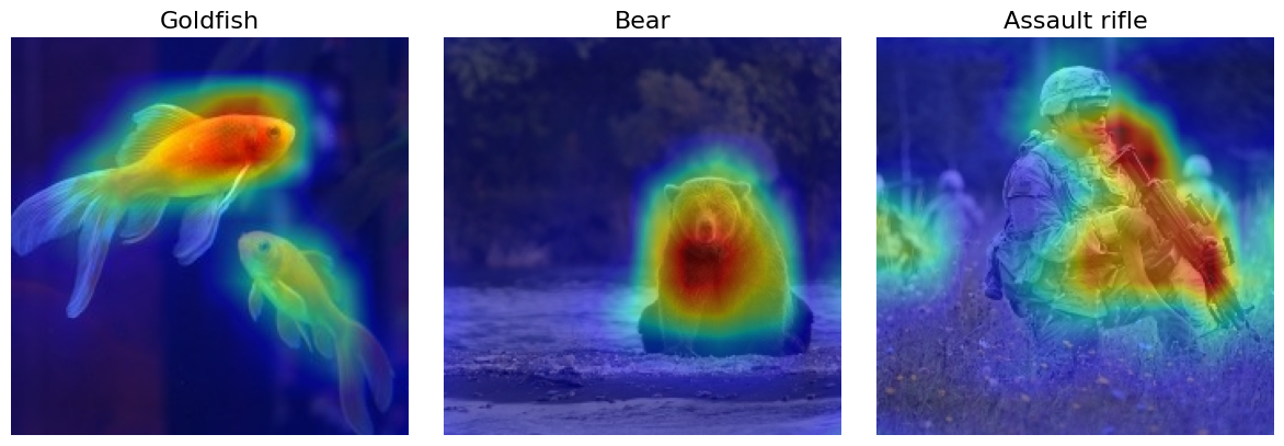
GradCAM++

GradCAM++ can provide better visual explanations of CNN model predictions.

[9]:

%%time

from tf_keras_vis.gradcam_plus_plus import GradcamPlusPlus

# Create GradCAM++ object
gradcam = GradcamPlusPlus(model, model_modifier=replace2linear, clone=True)

# Generate heatmap with GradCAM++
cam = gradcam(score, X, penultimate_layer=-1)

# Render
f, ax = plt.subplots(nrows=1, ncols=3, figsize=(12, 4))
for i, title in enumerate(image_titles):
    heatmap = np.uint8(cm.jet(cam[i])[..., :3] * 255)
    ax[i].set_title(title, fontsize=16)
    ax[i].imshow(images[i])
    ax[i].imshow(heatmap, cmap='jet', alpha=0.5)
    ax[i].axis('off')
plt.tight_layout()
plt.savefig('images/gradcam_plus_plus.png')
plt.show()

CPU times: user 14.9 s, sys: 1.98 s, total: 16.9 s
Wall time: 4.05 s

As you can see above, Now, the visualized attentions almost completely cover the target objects!

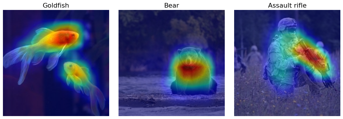
ScoreCAM

In the end, Here, we show you ScoreCAM. It is an another method that generates Class Activation Map. The characteristic of this method is that it’s the gradient-free method unlike GradCAM, GradCAM++ or Saliency.

[10]:

%%time

from tf_keras_vis.scorecam import Scorecam
from tf_keras_vis.utils import num_of_gpus

# Create ScoreCAM object
scorecam = Scorecam(model)

# Generate heatmap with ScoreCAM
cam = scorecam(score, X, penultimate_layer=-1)

# Render
f, ax = plt.subplots(nrows=1, ncols=3, figsize=(12, 4))
for i, title in enumerate(image_titles):
    heatmap = np.uint8(cm.jet(cam[i])[..., :3] * 255)
    ax[i].set_title(title, fontsize=16)
    ax[i].imshow(images[i])
    ax[i].imshow(heatmap, cmap='jet', alpha=0.5)
    ax[i].axis('off')
plt.tight_layout()
plt.show()

48/48 ━━━━━━━━━━━━━━━━━━━━ 207s 4s/step

CPU times: user 26min 17s, sys: 58.9 s, total: 27min 16s
Wall time: 3min 40s

As you can see above, The visualized images are more sophisticated!

Faster-ScoreCAM

ScoreCAM is a great method, however, it takes a bit more time to process it than other cam methods. There is a good news for us. Faster-ScorecAM that makes ScoreCAM to be more efficient was devised by @tabayashi0117.

https://github.com/tabayashi0117/Score-CAM/blob/master/README.md#faster-score-cam

We thought that several channels were dominant in generating the final heat map. Faster-Score-CAM adds the processing of “use only channels with large variances as mask images” to Score-CAM. (max_N = -1 is the original Score-CAM).

[11]:

%%time

from tf_keras_vis.scorecam import Scorecam

# Create ScoreCAM object
scorecam = Scorecam(model, model_modifier=replace2linear)

# Generate heatmap with Faster-ScoreCAM
cam = scorecam(score, X, penultimate_layer=-1, max_N=10)

# Render
f, ax = plt.subplots(nrows=1, ncols=3, figsize=(12, 4))
for i, title in enumerate(image_titles):
    heatmap = np.uint8(cm.jet(cam[i])[..., :3] * 255)
    ax[i].set_title(title, fontsize=16)
    ax[i].imshow(images[i])
    ax[i].imshow(heatmap, cmap='jet', alpha=0.5)
    ax[i].axis('off')
plt.tight_layout()
plt.show()

3/3 ━━━━━━━━━━━━━━━━━━━━ 13s 4s/step

CPU times: user 1min 41s, sys: 2.52 s, total: 1min 43s
Wall time: 14.8 s